Lab 6: Resistor Inductor Capacitor Series Circuits
Archie Wheeler
Michael McMearty
02.26.2012
A pdf version of this lab may downloaded here.
The odt version of this lab may be downloaded here.
Abstract
In this lab, we investigated the relationships between inductors, resistors, and capacitors when connected in parallel in a AC circuit. This lab took special consideration to noting the phase angles between the different voltages across each of the elements. The lab was a success, and our measured data seemed to hold up fairly well to equations that we were taught in the classroom. In this lab, we had considerable %error, which most likely arose from unmeasured resistances in the circuit, and an overall lack of precision.
Contents
Objectives
- To observe the relationships between the voltage and current across resistors, inductors, and capacitors in series combinations as the frequency of the source is varied.
- To observe resonance in an RLC circuit.
Methods
Part 1: LR Circuits
We set up our circuit board, connecting an AC signal generator in series with a 8.2mH inductor and a 10.02Ω resistor. For two different data runs, one with a metal bar in the inductor and another without the metal bar, we collected voltages and times at a sampling rate of 10000Hz over a period of 0.1s. We inspected a table of the data and found when each of the voltages crossed 0, and put those values in for the respective t values. Comparing these t values with omega, and several relationships outlined in the lab wiki, we were able to create graphs whose slope would give us certain ratios which could be compared to nominal resistances and inductances. In this way, we were able to find a %error.
Part 2: RC Circuits
We again set up our circuit board, but we ran the resistor in series with a 330μF resistor rather than the inductor. For five different frequencies, we collected voltages compared to time at a sampling rate of 10000Hz over a period of 0.1s. We calculated the phase angle φ and took the cotangent, which should equal RCω. With this relationship, we were able to create a graph, displaying the relationship nicely, and allowing us to find a %error.
Part 3: RLC Circuits
This time, we set up our circuit board with the resistor, inductor, and capacitor in series. We calculated the theoretical value for the resonant frequency using the values of capacitance and inductance. We then adjusted the frequency to be one fifth of the calculated theoretical value and measured the maximum and root mean squared voltage for the circuit. We also graphically determined the phase angle between the source voltage and the voltage across the resistor. We then repeated this for a frequency five times the resonant frequency, and then found the resonant frequency by adjusting the signal frequency. This frequency was then recorded as the resonant frequency.
We then inserted the metal rod through the inductor to increase its inductance. The process was repeated in order to find values for phase angles and maximum and rms voltages for frequencies of one, one fifth, and five times the resonant frequency.
Setup
Materials:- Cables, 3, with din connectors
- Pasco Signal Generator PI-9587
- Pasco Circuit Board with 100 and 330 microfarad capacitors, 8 millihenry inductor having about 5Ω resistance, and a 10Ω resistor
- Multimeter
- Capacitance meter with 200 microfarad range
- Pasco Signal Interface Data Studio and Graphical Analysis software
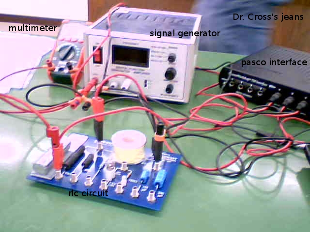
Our setup for part 1

Our setup for part 2

Our setup for part 3
Data and Analysis
Part 1 - Series RL Circuit

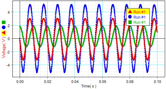
Voltage across resistor, inductor, and signal generator vs. time at f=30Hz
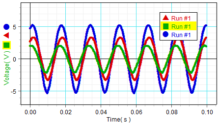
Voltage across resistor, inductor, and signal generator vs. time at f=60Hz

Voltage across resistor, inductor, and signal generator vs. time at f=100Hz

Voltage across resistor, inductor, and signal generator vs. time at f=150Hz

Voltage across resistor, inductor, and signal generator vs. time at f=200Hz
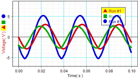
Voltage across resistor, inductor, and signal generator vs. time at f=30Hz with a metal bar in the inductor
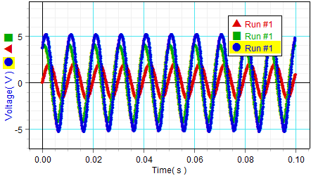
Voltage across resistor, inductor, and signal generator vs. time at f=100Hz with a metal bar in the inductor

Voltage across resistor, inductor, and signal generator vs. time at f=150Hz with a metal bar in the inductor

Voltage across resistor, inductor, and signal generator vs. time at f=200Hz with a metal bar in the inductor
Analysis: Part a - No bar in inductor 15:52
| f(Hz) | ω(rad/s) | tR(s) | tL | tS(s) | φL(rad) | φS(rad) | tan(φL) | tan(φS) |
|---|---|---|---|---|---|---|---|---|
| 30.15 | 189.4 | 0.0107 | 0.0930 | 0.0102 | -15.59 | 0.095 | 0.118 | 0.095 |
| 60.05 | 377.3 | 0.0062 | 0.0480 | 0.0057 | -15.77 | 0.189 | -0.063 | 0.191 |
| 100.1 | 628.9 | 0.0052 | 0.0040 | 0.0047 | 0.75 | 0.314 | 0.940 | 0.325 |
| 150 | 942.5 | 0.0049 | 0.0039 | 0.0044 | 0.94 | 0.471 | 1.376 | 0.510 |
| 200 | 1256.6 | 0.0039 | 0.0030 | 0.0034 | 1.13 | 0.628 | 2.125 | 0.727 |
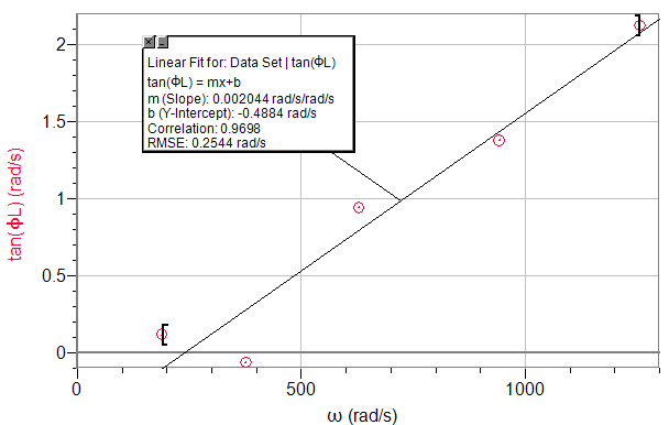
tan(φL) vs. ω

tan(φS) vs. ω
ΔV = 3.499
RResistor=10.2Ω
RInductor=5.6Ω
L=8.042mH
Graph 1
tan(φL)=(L/RL)ω
Slope = L/RL
Slope Experimental = 0.002044s
Slope Theoretical = 0.001436s
%Error = 39.6%
Graph 2
tan(φL)=(L/(R+RL))ω
Slope = L/(R+RL)
Slope Experimental = 0.0005889s
Slope Theoretical = 0.0005089s
%Error = 15.7%
Possible sources of error include a significant amount of resistance within the wire and battery, the heating up of a resistor, or a miscalibrated multimeter. I seriously suspect that in the first graph, the second data point was a mistake in recording the data, but by the time I had entered it in, we had already deleted the run, and I didn't want to set up everything again. Even though this point was off, it does not seem to affect the overall slope by that much.
Analysis: Part b - Bar in inductor 16:15
| f(Hz) | ω(rad/s) | tR(s) | tL(s) | tS(s) | φL(rad) | φS(rad) | tan(φL) | tan(φS) |
|---|---|---|---|---|---|---|---|---|
| 30.02 | 188.6 | 0.0151 | 0.0108 | 0.0131 | 0.8111 | 0.3772 | 1.052 | 0.3962 |
| 60.03 | 377.1 | 0.0092 | 0.0063 | 0.0074 | 1.093 | 0.6789 | 1.9350 | 0.8068 |
| 99.97 | 628.1 | 0.0053 | 0.0034 | 0.0040 | 1.193 | 0.8165 | 2.523 | 1.064 |
| 150 | 942.4 | 0.0054 | 0.0040 | 0.0043 | 1.319 | 1.036 | 3.894 | 1.690 |
| 200 | 1256.6 | 0.0046 | 0.0037 | 0.0038 | 1.1309 | 1.005 | 2.125 | 1.575 |

tan(φL) vs. ω

tan(φS) vs. ω
ΔV = 3.499
RResistor=10.2Ω
RInductor=5.6Ω
L=18.284mH
Graph 1
tan(φL)=(L/RL)ω
Slope = L/RL
Slope Experimental = 0.003504s
Slope Theoretical = 0.003257s
%Error = 7.58%
Graph 2
tan(φL)=(L/(R+RL))ω
Slope = L/(R+RL)
Slope Experimental = 0.001175s
Slope Theoretical = 0.001154s
%Error = 1.78%
Possible sources of error include a significant amount of resistance within the wire and battery, the heating up of a resistor, or a miscalibrated multimeter. In the first graph, I excluded the last point from my calculation, as it seemed to be an outlier.
Part 2 - Series RC Circuit
| f | ω | tR | tS | φS | cot φS | ωRC | %error |
|---|---|---|---|---|---|---|---|
| 20 | 125.6637 | 0.0039 | 0.0128 | -1.1134 | 0.4922 | 0.4023 | 22.36% |
| 30 | 188.4956 | 0.0250 | 0.0299 | -0.9236 | 0.7557 | 0.6034 | 25.24% |
| 50 | 314.1593 | 0.0201 | 0.0223 | -0.6912 | 1.2088 | 1.0057 | 20.19% |
| 80 | 502.6548 | 0.0254 | 0.0264 | -0.4825 | 1.9089 | 1.6092 | 18.63% |
| 150 | 942.4778 | 0.0978 | 0.0981 | -0.2922 | 3.3247 | 3.0172 | 10.19% |
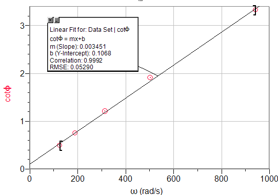
cot(φS) vs. ω. The slope of this line is expected to be RC.
R = 10.02Ω
C = 319.5μF
slopeExperimental=0.003451s
RC = 0.003201s
%Error=7.8%
We had to do this part twice. The first time we did it, we were only using 3 significant figures for our t values. Normally, 3 significant figures is more than ample information to come up with a good result. However, when dealing with trigonometric functions, especially tangents and cotangents, a difference in 0.0001s in this experiment can change the percent error by about 10%! We repeated the experiment by looking at the data points near 0, and guessing at exactly what time it actually crosses 0. With this extra accuracy, we were able to really hone in on the correct RC value
However, our measured results were consistently too high compared to our expected data. This could be due to extra resistance in the system. By playing with the numbers, one can see that the %error greatly diminishes as the resistance increases for our data. Thus, if there is extra unmeasured resistance in the system, that may well be the cause of our error.
| f | ω | VR0 | VC0 | VR0/VC0 |
|---|---|---|---|---|
| 19.96 | 125.4 | 2.06 | 4.76 | 0.43 |
| 30.00 | 188.5 | 2.72 | 4.39 | 0.62 |
| 50.06 | 314.5 | 3.60 | 3.64 | 0.99 |
| 80.01 | 502.7 | 4.12 | 2.82 | 1.46 |
| 150.00 | 942.5 | 4.53 | 1.81 | 2.50 |

Ratio of VR0/VC0 vs. ω. The slope is expected to be RC
R = 10.02Ω
C = 319.5μF
slopeExperimental=0.002660s
RC = 0.003201s
%Error=16.91%
%Error from other approach=22.92%
The ratio is quite a bit lower than what we would expect. One possible explanation could be that the measured resistance of the resistor was only part of the actual resistance. However, I have no proof for this. AC current still strikes me with wonder.
Part 3 - Series RLC Circuit
Part a: No rod

A graph of voltage vs. time at ω0=5 times the resonance
A graph of volate vs. time at ω0=resonance
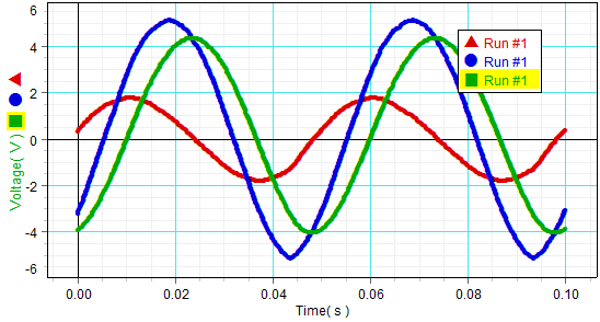
A graph of voltage vs. time ω0=1/5 times the resonance
| Frequency | Vmax | Vrms | φ |
|---|---|---|---|
| 0.2ω0 | 1.768 | 1.251 | 1.05 |
| 1ω0 | 3.008 | 2.201 | 0 |
| 5ω0 | 1.706 | 1.218 | 1.05 |
R=10.2Ω0
RL=5.6Ω
L=0.0231H
C=0.0003079F
ω0 theoretical=98.56Hz
ω0 experimental=~100Hz
%error = 1.46%
Part b: With rod

A graph of voltage vs. time at 5 times the resonance with a rod inserted into the inductor

A graph of voltage vs. time at ω=resonance with a rod inserted into the inductor

A graph of voltage vs. time at ω=1/5 times the resonance with a rod inserted into the inductor
| Frequency | Vmax | Vrms | φ |
|---|---|---|---|
| 0.2ω0 | 1.27 | 0.9 | 1.07 |
| 1ω0 | 2.78 | 2.016 | 0 |
| 5ω0 | 0.859 | 0.611 | 1.05 |
R=10.2Ω
RL=5.6Ω
L=0.0231H
C=0.0003079F
ω0 Theoretical 60.17Hz
ω0 Experimental ~45Hz
%error=25.21%
In the first RLC circuit, our predicted value for resonant frequency was almost exactly as predicted, but could not be determined with many significant figures as the adjustment of frequency to affect voltage was a rather crude method. Finding the maximum frequency was a rather guess and check method which is never as effective as a direct method.
Our measured value for resonant frequency in the second part was off by a magnitutde of about 1/4. Despite taking careful measurements of capacitance and inductance, we still had about 25% error. This source of this error may be due to a false reading of one of the elements, or because of some unexpected impedance by the multimeters and voltage sensors. However, this is likely to not be the case, as voltmeters have very high resistances (resonant frequency is independent of resistance(, ad would not be expected to have any capacitance or inductance. A possible explanation could be that the product of capacitance and inductance was calculated to be twice what it would have been. Given the equation for resonant frequency, this would cause the experimental error to be about 0.707 or sqrt(1/2) times the predicted theoretical error.
Our setup probably introduced some unknown capacitance or inductance which changed our calculation of resonant frequency
Conclusion
Overall, this lab was fairly successful. The relationships describing voltage drops and phase angles within an AC circuit were reasonably well proven by our results. Although our errors were much higher than we usually get, I am willing to blame those errors on things outside of our control to reasonably deal with.
One of the biggest challenges in getting reasonable data came in the difficulty to get an accurate time value for graphs crossing ΔV=0. In part 2, our first run failed largely because our results only contained figures accurate to 3 significant figures. While three significant figures is usually more than sufficient to come to conclusive results, when dealing with trigonometric functions, especially tangents, a difference of 0.0001s in a time value can make a huge difference, up to 10%!
I have a feeling that there was significant resistance elsewhere in the circuit that we did not account for. Perhaps the resistance within the Voltage Sensors and any nodes in the circuit was significant enough to skew the results by a few percent.
Several of the ways this lab could be improved would be if we used a slower frequency in the signal generator across more extreme elements. In this way, precision errors would not be so big of a deal. A wider variety of ω would also give us a wider spread of cotφ, which could also remove some error.
Signature

Archie Wheeler
02.28.12